Practical 8
In this practical we will will practice Pandas.
Libraries installation
First things first. Let’s start off by installing the required libraries. In particular we will need three libraries. Try and see if they are already available by typing the following commands in the console or put them in a python script:
import pandas as pd
import matplotlib.pyplot as plt
import numpy as np
if, upon execution, you do not get any error messages, you are sorted. Otherwise, you need to install them.
In Linux you can install the libraries by typing in a terminal
sudo pip3 install matplotlib, sudo pip3 install pandas and
sudo pip3 install numpy (or
sudo python3.X -m pip install matplotlib,
sudo python3.X -m pip install pandas and
sudo python3.X -m pip install numpy), where X is your python
version.
In Windows you can install the libraries by typing in the command
prompt (to open it type cmd in the search)
pip3 install matplotlib, pip3 install pandas and
pip3 install numpy. If you are using anaconda you need to run these
commands from the anaconda prompt.
Please install them in this order. You might not need to install numpy as matplotlib requires it. Once done that, try to perform the above imports again and they should work this time around.
Pandas
Pandas (the name comes from panel data) is a very efficient library to deal with numerical tables and time series. It is a quite complex library and here we will only scratch the surface of it. You can find a lot of information including the documentation on the Pandas website.
In particular the library pandas provides two data structures: Series and DataFrames.
Series
Series are 1-dimensional structures (like lists) containing data. Series are characterized by two types of information: the values and the index (a list of labels associated to the data), therefore they are a bit like a list and a bit like a dictionary. The index is optional and can be added by the library if not specified.
How to define and access a Series
There are several ways to define a Series. We can specify both the values and the index esplicitly, or through a dictionary, or let python add the default index for us. We can access the index with the Series.index method and the values with the Series.values.
In [1]:
import pandas as pd
import random

print("Values and index explicitly defined")
#values and index explicitely defined
S = pd.Series([random.randint(0,20) for x in range(0,10)],
              index = list("ABCDEFGHIL"))

print(S)
print("The index:", S.index)
print("The values:", S.values)

print("------------------------\n")
print("From dictionary")
#from a dictionary
S1 = pd.Series({"one" : 1, "two" : 2, "ten": 10,
                "three" : 3, "four": 4, "forty" : 40})
print(S1)
print(S1.index)
print(S1.values)
print("------------------------\n")
print("Default index")
#index added by default
myData = [random.randint(0,10) for x in range(10)]
S2 = pd.Series(myData)

print(S2)
print(S2.index)
print(S2.values)

print("------------------------\n")
print("Same value repeated")
S3 = pd.Series(1.27, range(10))
print(S3)
print(S3.index)
print(S3.values)
Values and index explicitly defined
A     9
B     6
C    20
D    10
E     0
F    13
G    10
H     4
I    14
L    15
dtype: int64
The index: Index(['A', 'B', 'C', 'D', 'E', 'F', 'G', 'H', 'I', 'L'], dtype='object')
The values: [ 9  6 20 10  0 13 10  4 14 15]
------------------------

From dictionary
one       1
two       2
ten      10
three     3
four      4
forty    40
dtype: int64
Index(['one', 'two', 'ten', 'three', 'four', 'forty'], dtype='object')
[ 1  2 10  3  4 40]
------------------------

Default index
0     8
1     2
2     8
3    10
4     1
5     5
6     3
7     8
8     9
9     5
dtype: int64
RangeIndex(start=0, stop=10, step=1)
[ 8  2  8 10  1  5  3  8  9  5]
------------------------

Same value repeated
0    1.27
1    1.27
2    1.27
3    1.27
4    1.27
5    1.27
6    1.27
7    1.27
8    1.27
9    1.27
dtype: float64
RangeIndex(start=0, stop=10, step=1)
[1.27 1.27 1.27 1.27 1.27 1.27 1.27 1.27 1.27 1.27]
Data in a series can be accessed by using the label (i.e. the index)
as in a dictionary or through its position as in a list. Slicing is
also allowed both by position and index. In the latter case, we
can do Series[S:E] with S and E indexes, both S and E are
included.
It is also possible to retrieve some elements by passing a list of positions or indexes. Head and tail methods can also be used to retrieve the top or bottom N elements with Series.head(N) or Series.tail(N).
In [3]:
import pandas as pd
import random

#values and index explicitely defined
S = pd.Series([random.randint(0,20) for x in range(0,10)],
              index = list("ABCDEFGHIL"))
print(S)
print("")

print("Value at label \"A\":", S["A"])
print("Value at index 1:", S[1])
print("")

print("Slicing from 1 to 3:") #note 3 excluded
print(S[1:3])
print("")
print("Slicing from C to H:") #note H included!
print(S["C":"H"])
print("")

print("Retrieving from list:")
print(S[[1,3,5,7,9]])
print(S[["A","C","E","G"]])
print("")

print("Top 3")
print(S.head(3))
print("")
print("Bottom 3")
print(S.tail(3))
A    15
B    11
C     4
D     7
E     1
F     4
G    15
H    14
I    14
L    17
dtype: int64

Value at label "A": 15
Value at index 1: 11

Slicing from 1 to 3:
B    11
C     4
dtype: int64

Slicing from C to H:
C     4
D     7
E     1
F     4
G    15
H    14
dtype: int64

Retrieving from list:
B    11
D     7
F     4
H    14
L    17
dtype: int64
A    15
C     4
E     1
G    15
dtype: int64

Top 3
A    15
B    11
C     4
dtype: int64

Bottom 3
H    14
I    14
L    17
dtype: int64
Operator broadcasting
Operations can automatically be broadcast to the entire Series. This is a quite cool feature and saves us from looping through the elements of the Series.
Example: Given a list of 10 integers and we want to divide them by 2. Without using pandas we would:
In [4]:
import random

listS = [random.randint(0,20) for x in range(0,10)]

print(listS)

for el in range(0,len(listS)):
    listS[el] /=2  #compact of X = X / 2

print(listS)
[6, 4, 5, 19, 14, 16, 9, 3, 13, 11]
[3.0, 2.0, 2.5, 9.5, 7.0, 8.0, 4.5, 1.5, 6.5, 5.5]
With pandas instead:
In [5]:
import pandas as pd
import random

S = pd.Series([random.randint(0,20) for x in range(0,10)],
              index = list("ABCDEFGHIL"))

print(S)
print("")
S1 = S / 2
print(S1)
A     4
B    13
C    14
D     6
E    13
F     2
G    13
H    19
I    20
L     7
dtype: int64

A     2.0
B     6.5
C     7.0
D     3.0
E     6.5
F     1.0
G     6.5
H     9.5
I    10.0
L     3.5
dtype: float64
Filtering
We can also apply boolean operators to obtain only the sub-Series with all the values satisfying a specific condition. This allows us to filter the Series.
Calling the boolean operator on the series alone (e.g. S > 10) will return a Series with True at the indexes where the condition is met, False at the others. Passing such a Series to a Series of the same lenght will return only the elements where the condition is True. Check the code below to see this in action.
In [6]:
import pandas as pd
import random

S = pd.Series([random.randint(0,20) for x in range(0,10)],
              index = list("ABCDEFGHIL"))

print(S)
print("")
S1 = S>10
print(S1)
print("")
S2 = S[S > 10]
print(S2)
A    14
B    18
C    10
D     6
E    17
F    14
G     2
H    17
I     4
L    15
dtype: int64

A     True
B     True
C    False
D    False
E     True
F     True
G    False
H     True
I    False
L     True
dtype: bool

A    14
B    18
E    17
F    14
H    17
L    15
dtype: int64
Missing data
Operations involving Series might have to deal with missing data or non-valid values (both cases are represented as NaN, that is not a number). Operations are carried out by aligning the Series based on their indexes. Indexes not in common end up in NaN values. Although most the operations that can be performed on series quite happily deal with NaNs, it is possible to drop NaN values or to fill them (i.e. replace their value with some other value). The sytax is:
Series.dropna()
or
Series.fillna(some_value)
Note that these operations do not modify the Series but rather return a new Series.
In [7]:
import pandas as pd
import random

S = pd.Series([random.randint(0,10) for x in range(0,10)],
              index = list("ABCDEFGHIL"))

S1 = pd.Series([random.randint(0,10) for x in range(0,8)],
              index = list("DEFGHAZY"))

print("The dimensions of these Series:", S.shape)
print("")
print(S1)
print("---- S + S1 ----")
Ssum = S + S1
print(Ssum)
print("---- Dropping NaNs ----")
print(Ssum.dropna())
print("---- Filling NaNs ----")
print(Ssum.fillna("my_value"))
The dimensions of these Series: (10,)

D     4
E     2
F     7
G     2
H     0
A     6
Z     1
Y    10
dtype: int64
---- S + S1 ----
A    10.0
B     NaN
C     NaN
D    14.0
E     4.0
F    14.0
G     8.0
H     1.0
I     NaN
L     NaN
Y     NaN
Z     NaN
dtype: float64
---- Dropping NaNs ----
A    10.0
D    14.0
E     4.0
F    14.0
G     8.0
H     1.0
dtype: float64
---- Filling NaNs ----
A          10
B    my_value
C    my_value
D          14
E           4
F          14
G           8
H           1
I    my_value
L    my_value
Y    my_value
Z    my_value
dtype: object
Computing stats
Pandas offer several operators to compute stats on the data stored in a Series. These include basic stats like min, max (and relative indexes with argmin and argmax) mean, std, quantile (to get the quantiles. A description of the data can be obtained by using the method describe and the counts for each value can be obtained by value_counts. Other methods available are sum and cumsum (for the sum and cumulative sum of the elements), autocorr and corr (for autocorrelation and correlation) and many others. For a complete list check the Pandas reference.
Note: as said before, when these methods do not return a single value, they return a Series.
Example: Fill the previous Series with the mean values of the series rather than NaNs.
In [8]:
Ssum = S + S1
print(Ssum)
print("---- Filling with avg value ----")
print(Ssum.fillna(Ssum.mean()))
A    10.0
B     NaN
C     NaN
D    14.0
E     4.0
F    14.0
G     8.0
H     1.0
I     NaN
L     NaN
Y     NaN
Z     NaN
dtype: float64
---- Filling with avg value ----
A    10.0
B     8.5
C     8.5
D    14.0
E     4.0
F    14.0
G     8.0
H     1.0
I     8.5
L     8.5
Y     8.5
Z     8.5
dtype: float64
Let’s see some operators introduced above in action.
In [9]:
import pandas as pd
import random

S = pd.Series([random.randint(0,10) for x in range(0,10)],
              index = list("ABCDEFGHIL"))
print("The data:")
print(S)
print("")
print("Its description")
print(S.describe())
print("")
print("Specifying different quantiles:")
print(S.quantile([0.1,0.2,0.8,0.9]))
print("")
print("Histogram:")
print(S.value_counts())
print("")
print("The type is a Series:")
print(type(S.value_counts()))
print("Summing the values:")
print(S.sum())
print("")
print("The cumulative sum:")
print(S.cumsum())
The data:
A     3
B    10
C     3
D     4
E     9
F     9
G     5
H     0
I    10
L     5
dtype: int64

Its description
count    10.000000
mean      5.800000
std       3.489667
min       0.000000
25%       3.250000
50%       5.000000
75%       9.000000
max      10.000000
dtype: float64

Specifying different quantiles:
0.1     2.7
0.2     3.0
0.8     9.2
0.9    10.0
dtype: float64

Histogram:
10    2
9     2
5     2
3     2
4     1
0     1
dtype: int64

The type is a Series:
<class 'pandas.core.series.Series'>
Summing the values:
58

The cumulative sum:
A     3
B    13
C    16
D    20
E    29
F    38
G    43
H    43
I    53
L    58
dtype: int64
Example:
Create two Series from the lists [2, 4, 6, 8, 10, 12, 13, 14, 15, 16], [1, 3, 5, 7, 9, 11, 13, 14, 15, 16] using the same index for both: [‘9B47’, ‘468B’, ‘B228’, ‘3C52’, ‘AE2E’, ‘DFF6’, ‘C38B’, ‘2CE5’, ‘0325’, ‘398F’].
Let’s compare the distribution stats of the two Series (mean value, max, min, quantiles) and get the index and value of the positions where the two series are the same. Finally, let’s get the sub-series where the first has an higher value than the first quartile of the second and compute its stats.
In [10]:
import pandas as pd

L1 = [2, 4, 6, 8, 10, 12, 13, 14, 15, 16]
L2 = [1, 3, 5, 7, 9, 11, 13, 14, 15, 16]
I = ['9B47', '468B', 'B228', '3C52', 'AE2E', 'DFF6', 'C38B', '2CE5', '0325', '398F']
L1Series = pd.Series(L1,index = I)
L2Series = pd.Series(L2, index = I)
#Let's describe the stats
print("Stats of L1Series")
print(L1Series.describe())
print("")
print("Stats of L2Series")
print(L2Series.describe())
print("")
#This is a Series with boolean values (True means the two Series where the same)
Leq = L1Series == L2Series
print("Equality series")
print(Leq)
print("")
#Get the subseries where both are the same
Lsub = L1Series[Leq]
print("Subseries of identicals")
print(Lsub)
print("")
#Get the values that are the same
print("Identical values:")
print(Lsub.values)
print("")
#Get the indexes where the two series are the same
print("Indexes of identical values:")
print(Lsub.index)
print("")
firstQuartile = L2Series.quantile(0.25)
print("The first quartile of L2Series:",firstQuartile)
print("")
#Get the subseries in which L1 is bigger than L2
Lbig = L1Series[L1Series > firstQuartile]
print("The subseries with L1 > L2")
print(Lbig)
Stats of L1Series
count    10.000000
mean     10.000000
std       4.830459
min       2.000000
25%       6.500000
50%      11.000000
75%      13.750000
max      16.000000
dtype: float64

Stats of L2Series
count    10.00000
mean      9.40000
std       5.25357
min       1.00000
25%       5.50000
50%      10.00000
75%      13.75000
max      16.00000
dtype: float64

Equality series
9B47    False
468B    False
B228    False
3C52    False
AE2E    False
DFF6    False
C38B     True
2CE5     True
0325     True
398F     True
dtype: bool

Subseries of identicals
C38B    13
2CE5    14
0325    15
398F    16
dtype: int64

Identical values:
[13 14 15 16]

Indexes of identical values:
Index(['C38B', '2CE5', '0325', '398F'], dtype='object')

The first quartile of L2Series: 5.5

The subseries with L1 > L2
B228     6
3C52     8
AE2E    10
DFF6    12
C38B    13
2CE5    14
0325    15
398F    16
dtype: int64
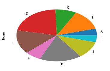
Plotting data
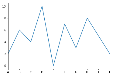
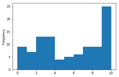
Using python’s matplotlib it is possible to plot data. The basic syntax
is Series.plot(kind = "type") the parameter kind can be used to
produce several types of plots (examples include line, hist,
pie, bar, see
here
for all possible choices). Note that matplotlib needs to be imported
and the pyplot needs to be shown with pyplot.show() to display the
plot.
In [11]:
import pandas as pd
import matplotlib.pyplot as plt
import random
S = pd.Series([random.randint(0,10) for x in range(0,10)],
              index = list("ABCDEFGHIL"))
print("The data:")
print(S)
S1 = pd.Series([random.randint(0,10) for x in range(0,100)])

S.plot()
plt.show()
plt.close()
S1.plot(kind = "hist")
plt.show()
plt.close()
S.plot(kind = "pie")
plt.show()
plt.close()
The data:
A     2
B     6
C     4
D    10
E     0
F     7
G     3
H     8
I     5
L     2
dtype: int64
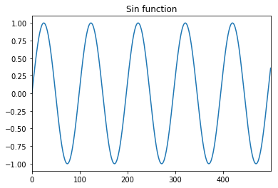
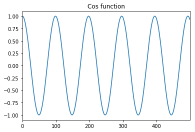
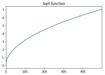
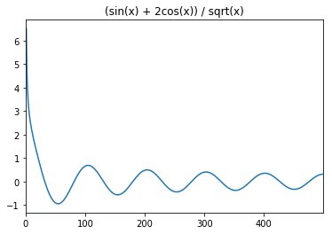
Example: Let’s create a series representing the sin, cos and sqrt functions and plot them.
In [6]:
import math
import matplotlib.pyplot as plt
import pandas as pd

x = [i/10 for i in range(0,500)]


y =  [math.sin(2*i/3.14 ) for i in x]
y1 = [math.cos(2*i/3.14 ) for i in x]
y2 = [math.sqrt(i) for i in x]
#print(x)

ySeries = pd.Series(y)
ySeries1 = pd.Series(y1)
ySeries2 = pd.Series(y2)

ySeries.plot()
plt.title("Sin function")
plt.show()
plt.close()
ySeries1.plot()
plt.title("Cos function")
plt.show()
plt.close()
ySeries2.plot()
plt.title("Sqrt function")
plt.show()
plt.close()
ySeries2 = (ySeries + 2*ySeries1)/ySeries2
ySeries2.plot()
plt.title("(sin(x) + 2cos(x)) / sqrt(x)")
plt.show()
Pandas DataFrames
DataFrames in pandas are the 2D analogous of Series. Dataframes are spreadsheet-like data structures with an ordered set of columns that can also be dishomogeneous. We can think about Dataframes as dictionaries of Series, each one representing a named column. Dataframes are described by an index that contains the labels of rows and a columns structure that holds the labels of the columns.
Note that the operation of extracting a column from a DataFrame returns a Series. Moreover, most (but not all!) of the operations that apply to Series also apply to DataFrames.
Define a DataFrame
There are several different ways to define a DataFrame. It is possible to create a DataFrame starting from a dictionary having Series as values. In this case, they keys of the dictionary are the columns of the DataFrame.
In [13]:
import pandas as pd

myData = {
    "temperature" : pd.Series([1, 3, 8, 13, 17, 20, 22, 22,18 ,13,6,2],
                            index = ["Jan","Feb", "Mar","Apr","May","Jun",
                                     "Jul","Aug","Sep","Oct","Nov","Dec"]
                             ),
    "dayLength" : pd.Series([9.7, 10.9, 12.5, 14.1, 15.6, 16.3, 15.9,
                             14.6,13,11.4,10,9.3],
                            index = ["Jan","Feb", "Mar","Apr","May","Jun",
                                     "Jul","Aug","Sep","Oct","Nov","Dec"]
                             )

}

DF = pd.DataFrame(myData)
print(DF)

print(DF.columns)
print(DF.index)
     dayLength  temperature
Jan        9.7            1
Feb       10.9            3
Mar       12.5            8
Apr       14.1           13
May       15.6           17
Jun       16.3           20
Jul       15.9           22
Aug       14.6           22
Sep       13.0           18
Oct       11.4           13
Nov       10.0            6
Dec        9.3            2
Index(['dayLength', 'temperature'], dtype='object')
Index(['Jan', 'Feb', 'Mar', 'Apr', 'May', 'Jun', 'Jul', 'Aug', 'Sep', 'Oct',
       'Nov', 'Dec'],
      dtype='object')
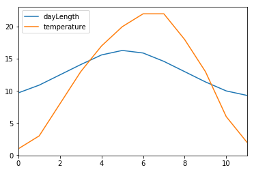
If the index is not specified, it is given by default:
In [14]:
import pandas as pd
import matplotlib.pyplot as plt
myData = {
"temperature" : pd.Series([1, 3, 8, 13, 17, 20,
22, 22,18 ,13,6,2]),
"dayLength" : pd.Series([9.7, 10.9, 12.5, 14.1, 15.6,
16.3,15.9,14.6,13,11.4,10,9.3])
}
DF = pd.DataFrame(myData)
print(DF)
print(DF.index)
DF.plot()
plt.show()
plt.close()
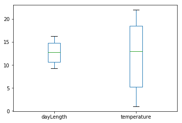
DF.plot(kind ="box")
plt.show()
    dayLength  temperature
0         9.7            1
1        10.9            3
2        12.5            8
3        14.1           13
4        15.6           17
5        16.3           20
6        15.9           22
7        14.6           22
8        13.0           18
9        11.4           13
10       10.0            6
11        9.3            2
RangeIndex(start=0, stop=12, step=1)
It is also possible to define a DataFrame from a list of dictionaries holding a set of values rather than Series. Note that when columns do not have the corresponding information a NaN is added. Indexes and columns can be changed after they have been defined.
In [15]:
import pandas as pd

myData = [{"A" : 1, "B" : 2, "C" : 3.2, "D" : 10},
          {"A" : 1, "B" : 2, "F" : 3.2, "G" : 10, "H":1},
          {"A" : 1, "B" : 2, "C" : 3.2, "D" : 1,
           "E": 4.1, "F" : 3.2, "G" : 10, "H":1}

         ]

DF = pd.DataFrame(myData)
print(DF)
print("")
#Let's change the columns and indexes
columns = "val1,val2,val3,val4,val5,val6,val7,val8".split(',')
inds = ["Day1", "Day2", "Day3"]

DF.columns = columns
DF.index = inds
print(DF)
   A  B    C     D    E    F     G    H
0  1  2  3.2  10.0  NaN  NaN   NaN  NaN
1  1  2  NaN   NaN  NaN  3.2  10.0  1.0
2  1  2  3.2   1.0  4.1  3.2  10.0  1.0

      val1  val2  val3  val4  val5  val6  val7  val8
Day1     1     2   3.2  10.0   NaN   NaN   NaN   NaN
Day2     1     2   NaN   NaN   NaN   3.2  10.0   1.0
Day3     1     2   3.2   1.0   4.1   3.2  10.0   1.0
Loading data from external files
Pandas also provide methods to load data from external files. In
particular, to load data from a .cvs file, we can use the method
pandas.read_csv(filename). This method has a lot of parameters, you
can see all the details on its usage on the official
documentation.
Some useful optional parameters are the separator (to specify the
column separator like sep="\t" for tab separated files), the
character to identify comments (comment="#") or that to skip some
lines (like the header for example or any initial comments to the file)
skiprows=N. The rows to use as column header can be specified with
the parameter header that accepts a number or a list of numbers.
Similarly, the columns to use as index can be specified with the
parameter index_col.
Other methods to read data in are pandas.read_excel(filename) that
works in a similar way but can load excel files (see
here).
Example: Let’s load the data stored in a csv datafile sampledata_orders.csv in a pandas DataFrame.
In [16]:
import pandas as pd

orders = pd.read_csv("file_samples/sampledata_orders.csv",
                     sep=",", index_col = 0, header = 0)
print("First 5 entries:")
print(orders.head())
print("")
print("The index:")
print(orders.index)
print("")
print("The column names:")
print(orders.columns)
print("")
print("A description of the numerical values:")
print(orders.describe())
First 5 entries:
        Order ID  Order Date Order Priority  Order Quantity       Sales  \
Row ID
1              3  10/13/2010            Low               6    261.5400
49           293   10/1/2012           High              49  10123.0200
50           293   10/1/2012           High              27    244.5700
80           483   7/10/2011           High              30   4965.7595
85           515   8/28/2010  Not Specified              19    394.2700

        Discount       Ship Mode   Profit  Unit Price  Shipping Cost  \
Row ID
1           0.04     Regular Air  -213.25       38.94          35.00
49          0.07  Delivery Truck   457.81      208.16          68.02
50          0.01     Regular Air    46.71        8.69           2.99
80          0.08     Regular Air  1198.97      195.99           3.99
85          0.08     Regular Air    30.94       21.78           5.94

             Customer Name Province   Region Customer Segment  \
Row ID
1       Muhammed MacIntyre  Nunavut  Nunavut   Small Business
49            Barry French  Nunavut  Nunavut         Consumer
50            Barry French  Nunavut  Nunavut         Consumer
80           Clay Rozendal  Nunavut  Nunavut        Corporate
85          Carlos Soltero  Nunavut  Nunavut         Consumer

       Product Category            Product Sub-Category  \
Row ID
1       Office Supplies          Storage & Organization
49      Office Supplies                      Appliances
50      Office Supplies  Binders and Binder Accessories
80           Technology    Telephones and Communication
85      Office Supplies                      Appliances

                                             Product Name Product Container  \
Row ID
1        Eldon Base for stackable storage shelf, platinum         Large Box
49      1.7 Cubic Foot Compact "Cube" Office Refrigera...        Jumbo Drum
50       Cardinal Slant-D® Ring Binder, Heavy Gauge Vinyl         Small Box
80                                                   R380         Small Box
85                               Holmes HEPA Air Purifier        Medium Box

        Product Base Margin   Ship Date
Row ID
1                      0.80  10/20/2010
49                     0.58   10/2/2012
50                     0.39   10/3/2012
80                     0.58   7/12/2011
85                     0.50   8/30/2010

The index:
Int64Index([   1,   49,   50,   80,   85,   86,   97,   98,  103,  107,
            ...
            6492, 6526, 6657, 7396, 7586, 7765, 7766, 7906, 7907, 7914],
           dtype='int64', name='Row ID', length=8399)

The column names:
Index(['Order ID', 'Order Date', 'Order Priority', 'Order Quantity', 'Sales',
       'Discount', 'Ship Mode', 'Profit', 'Unit Price', 'Shipping Cost',
       'Customer Name', 'Province', 'Region', 'Customer Segment',
       'Product Category', 'Product Sub-Category', 'Product Name',
       'Product Container', 'Product Base Margin', 'Ship Date'],
      dtype='object')

A description of the numerical values:
           Order ID  Order Quantity         Sales     Discount        Profit  \
count   8399.000000     8399.000000   8399.000000  8399.000000   8399.000000
mean   29965.179783       25.571735   1775.878179     0.049671    181.184423
std    17260.883447       14.481071   3585.050525     0.031823   1196.653372
min        3.000000        1.000000      2.240000     0.000000 -14140.700000
25%    15011.500000       13.000000    143.195000     0.020000    -83.315000
50%    29857.000000       26.000000    449.420000     0.050000     -1.500000
75%    44596.000000       38.000000   1709.320000     0.080000    162.750000
max    59973.000000       50.000000  89061.050000     0.250000  27220.690000

        Unit Price  Shipping Cost  Product Base Margin
count  8399.000000    8399.000000          8336.000000
mean     89.346259      12.838557             0.512513
std     290.354383      17.264052             0.135589
min       0.990000       0.490000             0.350000
25%       6.480000       3.300000             0.380000
50%      20.990000       6.070000             0.520000
75%      85.990000      13.990000             0.590000
max    6783.020000     164.730000             0.850000
Extract values by row and column
Once a DataFrame is populated we can access its content. Several options are available:
- Select by column
DataFrame[col]returns a Series - Select by row label
DataFrame.loc[row_label]returns a Series - Select row by integer location
DataFrame.iloc[row_position]returns a Series - Slice rows
DataFrame[S:E](S and E are labels, both included) returns a DataFrame - Select rows by boolean vector
DataFrame[bool_vect]returns a DataFrame
Note that if names are well formed (i.e. no spaces, no strange characters…) we can use DataFrame.col instead of DataFrame[col]. Here are some ways to extract data from the orders dataframe:
In [17]:
import pandas as pd

orders = pd.read_csv("file_samples/sampledata_orders.csv", sep=",", index_col =0, header=0)

print("The Order Quantity column (top 5)")
print(orders["Order Quantity"].head(5))
print("")
print("The Sales column (top 10)")
print(orders.Sales.head(10))
print("")
print("The row with ID:50")
r50 = orders.loc[50]
print(r50)
print("")
print("The third row:")
print(orders.iloc[3])

print("The Order Quantity, Sales, Discount and Profit of the 2nd,4th, 6th and 8th row:")
print(orders[1:8:2][["Order Quantity", "Sales","Discount", "Profit"]])
print("The Order Quantity, Sales, Discount and  Profit of orders with discount > 10%:")
print(orders[orders["Discount"] > 0.1][["Order Quantity", "Sales","Discount", "Profit"]])
The Order Quantity column (top 5)
Row ID
1      6
49    49
50    27
80    30
85    19
Name: Order Quantity, dtype: int64

The Sales column (top 10)
Row ID
1        261.5400
49     10123.0200
50       244.5700
80      4965.7595
85       394.2700
86       146.6900
97        93.5400
98       905.0800
103     2781.8200
107      228.4100
Name: Sales, dtype: float64

The row with ID:50
Order ID                                                             293
Order Date                                                     10/1/2012
Order Priority                                                      High
Order Quantity                                                        27
Sales                                                             244.57
Discount                                                            0.01
Ship Mode                                                    Regular Air
Profit                                                             46.71
Unit Price                                                          8.69
Shipping Cost                                                       2.99
Customer Name                                               Barry French
Province                                                         Nunavut
Region                                                           Nunavut
Customer Segment                                                Consumer
Product Category                                         Office Supplies
Product Sub-Category                      Binders and Binder Accessories
Product Name            Cardinal Slant-D® Ring Binder, Heavy Gauge Vinyl
Product Container                                              Small Box
Product Base Margin                                                 0.39
Ship Date                                                      10/3/2012
Name: 50, dtype: object

The third row:
Order ID                                         483
Order Date                                 7/10/2011
Order Priority                                  High
Order Quantity                                    30
Sales                                        4965.76
Discount                                        0.08
Ship Mode                                Regular Air
Profit                                       1198.97
Unit Price                                    195.99
Shipping Cost                                   3.99
Customer Name                          Clay Rozendal
Province                                     Nunavut
Region                                       Nunavut
Customer Segment                           Corporate
Product Category                          Technology
Product Sub-Category    Telephones and Communication
Product Name                                    R380
Product Container                          Small Box
Product Base Margin                             0.58
Ship Date                                  7/12/2011
Name: 80, dtype: object
The Order Quantity, Sales, Discount and Profit of the 2nd,4th, 6th and 8th row:
        Order Quantity       Sales  Discount   Profit
Row ID
49                  49  10123.0200      0.07   457.81
80                  30   4965.7595      0.08  1198.97
86                  21    146.6900      0.05     4.43
98                  22    905.0800      0.09   127.70
The Order Quantity, Sales, Discount and  Profit of orders with discount > 10%:
        Order Quantity    Sales  Discount  Profit
Row ID
176                 11  663.784      0.25 -481.04
3721                22  338.520      0.21  -17.75
37                  43  586.110      0.11   98.44
2234                 1   27.960      0.17   -9.13
4900                49  651.900      0.16  -74.51
Broadcasting, filtering and computing stats
These work pretty much like on Series and pandas takes care of adding NaNs when it cannot perform some operations due to missing values and so on.
Obviously some operators, when applied to entire tables might not always make sense (like mean or sum of strings).
In [18]:
import pandas as pd

orders = pd.read_csv("file_samples/sampledata_orders.csv", sep=",", index_col =0, header=0)

orders_10 = orders[["Sales","Profit", "Product Category"]].head(10)
orders_5 = orders[["Sales","Profit", "Product Category"]].head()
orders_20 = orders[["Sales","Profit", "Product Category"]].head(20)
print(orders_20)
print("")

#Summing over the entries, does not make sense but...
print("Top10 + Top5:")
print(orders_10 + orders_5)
print("")

prod_cost = orders_20["Sales"] - orders_20["Profit"]
print(prod_cost)

print("")
print("Technology orders")
print(orders_20[orders_20["Product Category"] == "Technology"])
print("")
print("Office Supplies positive profit")
print(orders_20[ (orders_20["Product Category"] == "Office Supplies") & (orders_20["Profit"] >0) ])
             Sales   Profit Product Category
Row ID
1         261.5400  -213.25  Office Supplies
49      10123.0200   457.81  Office Supplies
50        244.5700    46.71  Office Supplies
80       4965.7595  1198.97       Technology
85        394.2700    30.94  Office Supplies
86        146.6900     4.43        Furniture
97         93.5400   -54.04  Office Supplies
98        905.0800   127.70  Office Supplies
103      2781.8200  -695.26  Office Supplies
107       228.4100  -226.36  Office Supplies
127       196.8500  -166.85  Office Supplies
128       124.5600   -14.33  Office Supplies
134       716.8400   134.72  Office Supplies
135      1474.3300   114.46       Technology
149        80.6100    -4.72  Office Supplies
160      1815.4900   782.91        Furniture
161       248.2600    93.80  Office Supplies
175      4462.2300   440.72        Furniture
176       663.7840  -481.04        Furniture
203       834.9040   -11.68       Technology

Top10 + Top5:
            Sales   Profit                Product Category
Row ID
1         523.080  -426.50  Office SuppliesOffice Supplies
49      20246.040   915.62  Office SuppliesOffice Supplies
50        489.140    93.42  Office SuppliesOffice Supplies
80       9931.519  2397.94            TechnologyTechnology
85        788.540    61.88  Office SuppliesOffice Supplies
86            NaN      NaN                             NaN
97            NaN      NaN                             NaN
98            NaN      NaN                             NaN
103           NaN      NaN                             NaN
107           NaN      NaN                             NaN

Row ID
1       474.7900
49     9665.2100
50      197.8600
80     3766.7895
85      363.3300
86      142.2600
97      147.5800
98      777.3800
103    3477.0800
107     454.7700
127     363.7000
128     138.8900
134     582.1200
135    1359.8700
149      85.3300
160    1032.5800
161     154.4600
175    4021.5100
176    1144.8240
203     846.5840
dtype: float64

Technology orders
            Sales   Profit Product Category
Row ID
80      4965.7595  1198.97       Technology
135     1474.3300   114.46       Technology
203      834.9040   -11.68       Technology

Office Supplies positive profit
           Sales  Profit Product Category
Row ID
49      10123.02  457.81  Office Supplies
50        244.57   46.71  Office Supplies
85        394.27   30.94  Office Supplies
98        905.08  127.70  Office Supplies
134       716.84  134.72  Office Supplies
161       248.26   93.80  Office Supplies
Statistics can be computed by column (normally the default) or by
row (specifying axis=1) or on the entire table.
Here you can find the complete list of methods that can be applied.
In [19]:
import pandas as pd

data = pd.read_csv("file_samples/random.csv", sep=",", header=0)

print("Global description")
print(data.describe())
print("")

print(data)
print("")

print("Let's reduce A in [0,1]")
print(data["A"]/ data["A"].max())

print("Let's reduce first row in [0,1]")
print(data.iloc[0]/ data.loc[0].max())

print("Mean and std values (by column)")
print(data.mean())
print(data.std())
print("")
print("Mean and std values (by column) - top 10 values")
print(data.head(10).mean(axis=1))
print(data.head(10).std(axis=1))

print("Cumulative sum (by column)- top 10 rows")
print(data.head(10).cumsum())

print("Cumulative sum (by row) - top 10 rows")
print(data.head(10).cumsum(axis = 1 ))
Global description
               A          B           C          D           E          F  \
count  50.000000  50.000000   50.000000  50.000000   50.000000  50.000000
mean   45.240000  49.760000   54.120000  50.500000   57.860000  49.180000
std    28.393417  32.193015   25.165282  28.321226   32.443364  28.488229
min     0.000000   0.000000    5.000000   1.000000    2.000000   1.000000
25%    21.750000  18.000000   35.750000  28.250000   29.250000  25.000000
50%    42.000000  49.500000   52.500000  49.500000   68.000000  52.000000
75%    63.250000  76.250000   73.750000  76.000000   86.750000  75.500000
max    99.000000  99.000000  100.000000  95.000000  100.000000  97.000000

                G         H          I           L
count   50.000000  50.00000  50.000000   50.000000
mean    49.780000  47.78000  46.920000   51.780000
std     29.673248  29.75978  31.056788   30.613649
min      1.000000   1.00000   0.000000    3.000000
25%     26.500000  24.50000  19.000000   26.250000
50%     51.000000  42.50000  44.000000   46.500000
75%     76.750000  72.00000  73.000000   82.000000
max    100.000000  99.00000  98.000000  100.000000

     A   B    C   D    E   F    G   H   I    L
0   28  69    5  41   12  62   90  32  33   85
1   91  59   64  94    4  51   45  52  96    5
2   54  74   53  92   20  84   85  21  98   73
3   99   0   39  12   90  15   62  38   4   67
4   98  10   35  77   46  97   88  72  15   37
5   44   9   91  57   98  63   52  77  62    7
6   76  17   12  41   69  34  100  29   0   91
7   52  25   43  59   87  91    1  90  23   90
8   56  33   38  91   13   1   34  17  22   82
9   29  18   42  48   34  16   64   7  46    9
10  81  77   38  93   63  90   57  58  52  100
11  57  97   23  59   38  93   46  49  88   86
12  57   0   79  78  100  76   16  31  79    8
13  18   1   67  44    2  17   53  51   6   23
14  77  95   94  88    9  25   54  23  36   35
15  87  42   63  33   95  53   11  58  53    3
16  34  24   24  28   74  79   86  98  42   90
17   1  31   20  63   70   3   29  39   5   87
18  35  17   77  15    9  63   86  95  95   21
19   0  85   13  13   60  74   44  78   7   56
20  61  20   47  21   85  78   53  14  37   70
21  81  15   89  54   38  59   72  35  59   12
22  20  81   76  15   64  18    9  47  11   81
23  57  94   73  19   21  79   81  45  71   40
24   2  58   83  67   99  46   76  70  50   45
25  64  13   52  60   32  70   32   4  73   20
26  27  49  100  48   70  30   58  48  42   36
27  82  89   93  73   30  64   18  54  93   82
28  19  85   98   7   84  71   77  20  18   63
29  34  95   68  23   68  38   73   1  28   10
30  33  60   66  80   94  41   53  99  29   57
31   0  99   18   2   29  28   11  30  36   56
32  20  61   33  89   52  59   50  55   4   33
33  82  72   41  33   92  16   18  99  73   91
34   8  28   22  29   83  53   47  10  42   34
35  64  50   24  59    6  83   92  91  87   98
36  42  73   50  17   91   9   39  37  97   50
37  27  49   67  61   21  25   94  96  16   98
38  44  44   48  70   86  85    9  31   4   46
39  36  93   64   1   96  89   14  75  10   84
40  20  13   34  87   11  10    2   5  91   27
41  54   2   61  80   98  53   96  40   2   26
42  42  88   79  31   41  23   50  95  77   26
43   7  14   56  95   70  28   78  31  34   95
44  40  65   34  44   97  36    3  90  55   13
45  97  61   45  32   91  26   84  33  57   80
46  60  49   47  92   81  51    7  18  66   47
47  39  98   90  33   68   5   26  72  76   37
48   6  18   74  51   77  19   28  21  81   46
49  20  69   54  26   25  80   36   8  65   31

Let's reduce A in [0,1]
0     0.282828
1     0.919192
2     0.545455
3     1.000000
4     0.989899
5     0.444444
6     0.767677
7     0.525253
8     0.565657
9     0.292929
10    0.818182
11    0.575758
12    0.575758
13    0.181818
14    0.777778
15    0.878788
16    0.343434
17    0.010101
18    0.353535
19    0.000000
20    0.616162
21    0.818182
22    0.202020
23    0.575758
24    0.020202
25    0.646465
26    0.272727
27    0.828283
28    0.191919
29    0.343434
30    0.333333
31    0.000000
32    0.202020
33    0.828283
34    0.080808
35    0.646465
36    0.424242
37    0.272727
38    0.444444
39    0.363636
40    0.202020
41    0.545455
42    0.424242
43    0.070707
44    0.404040
45    0.979798
46    0.606061
47    0.393939
48    0.060606
49    0.202020
Name: A, dtype: float64
Let's reduce first row in [0,1]
A    0.311111
B    0.766667
C    0.055556
D    0.455556
E    0.133333
F    0.688889
G    1.000000
H    0.355556
I    0.366667
L    0.944444
Name: 0, dtype: float64
Mean and std values (by column)
A    45.24
B    49.76
C    54.12
D    50.50
E    57.86
F    49.18
G    49.78
H    47.78
I    46.92
L    51.78
dtype: float64
A    28.393417
B    32.193015
C    25.165282
D    28.321226
E    32.443364
F    28.488229
G    29.673248
H    29.759780
I    31.056788
L    30.613649
dtype: float64

Mean and std values (by column) - top 10 values
0    45.7
1    56.1
2    65.4
3    42.6
4    57.5
5    56.0
6    46.9
7    56.1
8    38.7
9    31.3
dtype: float64
0    29.424291
1    33.013297
2    27.785688
3    35.647035
4    33.069792
5    30.342489
6    34.853503
7    32.942543
8    29.431842
9    18.826990
dtype: float64
Cumulative sum (by column)- top 10 rows
     A    B    C    D    E    F    G    H    I    L
0   28   69    5   41   12   62   90   32   33   85
1  119  128   69  135   16  113  135   84  129   90
2  173  202  122  227   36  197  220  105  227  163
3  272  202  161  239  126  212  282  143  231  230
4  370  212  196  316  172  309  370  215  246  267
5  414  221  287  373  270  372  422  292  308  274
6  490  238  299  414  339  406  522  321  308  365
7  542  263  342  473  426  497  523  411  331  455
8  598  296  380  564  439  498  557  428  353  537
9  627  314  422  612  473  514  621  435  399  546
Cumulative sum (by row) - top 10 rows
    A    B    C    D    E    F    G    H    I    L
0  28   97  102  143  155  217  307  339  372  457
1  91  150  214  308  312  363  408  460  556  561
2  54  128  181  273  293  377  462  483  581  654
3  99   99  138  150  240  255  317  355  359  426
4  98  108  143  220  266  363  451  523  538  575
5  44   53  144  201  299  362  414  491  553  560
6  76   93  105  146  215  249  349  378  378  469
7  52   77  120  179  266  357  358  448  471  561
8  56   89  127  218  231  232  266  283  305  387
9  29   47   89  137  171  187  251  258  304  313
Merging DataFrames
It is possible to merge together DataFrames having a common column name.
The merge can be done with the pandas merge method. Upon merging,
the two tables will be concatenated into a bigger one containing
information from both DataFrames. The basic syntax is:
pandas.merge(DataFrame1, DataFrame2, on="col_name", how="inner/outer/left/right")
The column on which perform the merge is specified with the parameter
on followed by the column name, while the behaviour of the merging
depends on the parameter how that tells pandas how to behave when
dealing with non-matching data. In particular:
1. how = inner : non-matching entries are discarded;
2. how = left : ids are taken from the first DataFrame;
3. how = right : ids are taken from the second DataFrame;
4. how = outer : ids from both are retained.
In [20]:
import pandas as pd

Snp1 = {"id": ["SNP_FB_0411211","SNP_FB_0412425","SNP_FB_0942385",
               "CH01f09","Hi05f12x","SNP_FB_0942712" ],
        "type" : ["SNP","SNP","SNP","SSR","SSR","SNP"]
       }
Snp2 = {"id" : ["SNP_FB_0411211","SNP_FB_0412425",
                "SNP_FB_0942385", "CH01f09","SNP_FB_0428218" ],
      "chr" : ["1", "15","7","9","1"]
     }

DFs1 = pd.DataFrame(Snp1)
DFs2 = pd.DataFrame(Snp2)

print(DFs1)
print(DFs2)
print("")
print("Inner merge (only common in both)")
inJ = pd.merge(DFs1,DFs2, on = "id", how = "inner")
print(inJ)
print("")
print("Left merge (IDS from DFs1)")
leftJ = pd.merge(DFs1,DFs2, on = "id", how = "left")
print(leftJ)
print("")
print("Right merge (IDS from DFs2)")
rightJ = pd.merge(DFs1,DFs2, on = "id", how = "right")
print(rightJ)
print("")
print("Outer merge (IDS from both)")
outJ = pd.merge(DFs1,DFs2, on = "id", how = "outer")
print(outJ)
               id type
0  SNP_FB_0411211  SNP
1  SNP_FB_0412425  SNP
2  SNP_FB_0942385  SNP
3         CH01f09  SSR
4        Hi05f12x  SSR
5  SNP_FB_0942712  SNP
  chr              id
0   1  SNP_FB_0411211
1  15  SNP_FB_0412425
2   7  SNP_FB_0942385
3   9         CH01f09
4   1  SNP_FB_0428218

Inner merge (only common in both)
               id type chr
0  SNP_FB_0411211  SNP   1
1  SNP_FB_0412425  SNP  15
2  SNP_FB_0942385  SNP   7
3         CH01f09  SSR   9

Left merge (IDS from DFs1)
               id type  chr
0  SNP_FB_0411211  SNP    1
1  SNP_FB_0412425  SNP   15
2  SNP_FB_0942385  SNP    7
3         CH01f09  SSR    9
4        Hi05f12x  SSR  NaN
5  SNP_FB_0942712  SNP  NaN

Right merge (IDS from DFs2)
               id type chr
0  SNP_FB_0411211  SNP   1
1  SNP_FB_0412425  SNP  15
2  SNP_FB_0942385  SNP   7
3         CH01f09  SSR   9
4  SNP_FB_0428218  NaN   1

Outer merge (IDS from both)
               id type  chr
0  SNP_FB_0411211  SNP    1
1  SNP_FB_0412425  SNP   15
2  SNP_FB_0942385  SNP    7
3         CH01f09  SSR    9
4        Hi05f12x  SSR  NaN
5  SNP_FB_0942712  SNP  NaN
6  SNP_FB_0428218  NaN    1
Note that the columns we merge on do not necessarily need to be the
same, we can specify a correspondence between the row of the first
dataframe (the one on the left) and the second dataframe (the one on the
right) specifying which columns must have the same values to perform the
merge. This can be done by using the parameters
right_on = column_name and left_on = column_name:
In [9]:
%reset -s -f

import pandas as pd

d = dict({"A" : [1,2,3,4], "B" : [3,4,73,13]})
d2 = dict({"E" : [1,4,3,13], "F" : [3,1,71,1]})

DF = pd.DataFrame(d)
DF2 = pd.DataFrame(d2)

merged_onBE = DF.merge(DF2, left_on = 'B', right_on = 'E', how = "inner")
merged_onAF = DF.merge(DF2, right_on = "F", left_on = "A", how = "outer")
print("DF:")
print(DF)
print("DF2:")
print(DF2)
print("\ninner merge on BE")
print(merged_onBE)
print("\nouter merge on AF:")
print(merged_onAF)
DF:
   A   B
0  1   3
1  2   4
2  3  73
3  4  13
DF2:
    E   F
0   1   3
1   4   1
2   3  71
3  13   1

inner merge on BE
   A   B   E   F
0  1   3   3  71
1  2   4   4   1
2  4  13  13   1

outer merge on AF:
     A     B     E     F
0  1.0   3.0   4.0   1.0
1  1.0   3.0  13.0   1.0
2  2.0   4.0   NaN   NaN
3  3.0  73.0   1.0   3.0
4  4.0  13.0   NaN   NaN
5  NaN   NaN   3.0  71.0
Grouping
Given a DataFrame, it is possible to apply the so called split-apply-aggregate processing method. Basically, this helps to group the data according to the value of some columns, apply a function on the different groups and aggregate the results in a new DataFrame.
Grouping of a DataFrame can be done by using the
DataFrame.groupby(columnName) method which returns a
pandas.DataFrameGroupBy object, which basically is composed of two
information the name shared by each group and a DataFrame
containing all the elements belonging to that group.
Given a grouped DataFrame, each group can be obtained with the get_group(groupName) it is also possible to loop over the groups:
for groupName, groupDataFrame in grouped:
    #do something
It is also possible to aggregate the groups by applying some functions to each of them (please refer to the documentation).
Let’s see these things in action.
Example Given a list of labels and integers group them by label and compute the mean of all values in each group.
In [18]:
import pandas as pd

test = {"x": ["a","a", "b", "b", "c", "c" ],
        "y" : [2,4,0,5,5,10]
       }

DF = pd.DataFrame(test)
print(DF)
print("")
gDF = DF.groupby("x")
for i,g in gDF:
    print("Group: ", i)
    print(g)
    print(type(g))

aggDF = gDF.aggregate(pd.DataFrame.mean)
print(aggDF)
   x   y
0  a   2
1  a   4
2  b   0
3  b   5
4  c   5
5  c  10

Group:  a
   x  y
0  a  2
1  a  4
<class 'pandas.core.frame.DataFrame'>
Group:  b
   x  y
2  b  0
3  b  5
<class 'pandas.core.frame.DataFrame'>
Group:  c
   x   y
4  c   5
5  c  10
<class 'pandas.core.frame.DataFrame'>
     y
x
a  3.0
b  2.5
c  7.5
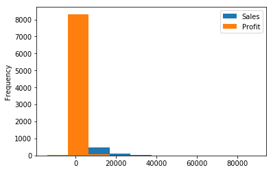
Example Given the orders data seen above, let’s get the columns “Sales”, “Profit” and “Product Category” and compute the total sum and the mean of the sales and profits for each product category.
In [21]:
import pandas as pd
import matplotlib.pyplot as plt

orders = pd.read_csv("file_samples/sampledata_orders.csv", sep=",",
                     index_col =0, header=0)

SPC = orders[["Sales","Profit", "Product Category"]]
print(SPC.head())

SPC.plot(kind = "hist", bins = 10)
plt.show()

print("")
grouped = SPC.groupby("Product Category")
for i,g in grouped:
    print("Group: ", i)

print("")
print("Count elements per category:") #get the series corresponding to the column
                                      #and apply the value_counts() method
print(orders["Product Category"].value_counts())
print("")
print("Total values:")
print(grouped.aggregate(pd.DataFrame.sum)[["Sales"]])

print("Mean values (sorted by profit):")
mv_sorted = grouped.aggregate(pd.DataFrame.mean).sort_values(by="Profit")
print(mv_sorted)
print("")
print("The most profitable is {}".format(mv_sorted.index[-1]))
             Sales   Profit Product Category
Row ID
1         261.5400  -213.25  Office Supplies
49      10123.0200   457.81  Office Supplies
50        244.5700    46.71  Office Supplies
80       4965.7595  1198.97       Technology
85        394.2700    30.94  Office Supplies
Group:  Furniture
Group:  Office Supplies
Group:  Technology

Count elements per category:
Office Supplies    4610
Technology         2065
Furniture          1724
Name: Product Category, dtype: int64

Total values:
                        Sales
Product Category
Furniture         5178590.542
Office Supplies   3752762.100
Technology        5984248.182
Mean values (sorted by profit):
                        Sales      Profit
Product Category
Furniture         3003.822820   68.116607
Office Supplies    814.048178  112.369072
Technology        2897.941008  429.207516

The most profitable is Technology
Exercises
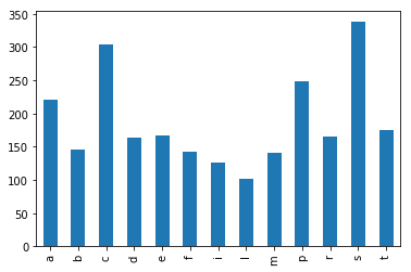
- The file top_3000_words.txt is a one-column file representing the top 3000 English words. Read the file and for each letter, count how many words start with that letter. Store this information in a dictionary. Create a pandas series from the dictionary and plot an histogram of all initials counting more than 100 words starting with them.
Show/Hide Solution
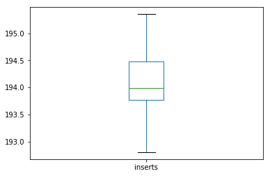
- The file filt_aligns.tsv is a tab separated value file representing alignments of paired-end reads on some apple chromosomes. Paired end reads have the property of being X bases apart from each other as they have been sequenced from the two ends of some size-selected DNA molecules.
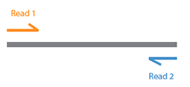
Each line of the file has the following information
readID\tChrPE1\tAlignmentPosition1\tChrPE2\tAlignmentPosition2. The
two ends of the same pair have the same readID. Load the read pairs
aligning on the same chromosome into two dictionaries. The first
(inserts) having readID as keys and the insert size (i.e. the
absolute value of AlignmentPosition1 - AlignmentPosition2) as value. The
second dictionary (chrs)will have readID as key and chromosome ID as
value. Example:
readID Chr11 31120 Chr11 31472
readID1 Chr7 12000 Chr11 11680
will result in:
inserts = {"readID" : 352, "readID1" : 320}
chrs = {"readID" : "Chr11", "readID1" : "Chr7"}
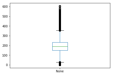
Once you have the two dictionaries:
1. Create a Series with all the insert sizes and show some
of its stats with the method **describe**. What is the mean
insert size? How many paried end are we using to create
this distribution?
2. Display the first 5 values of the series
3. Make a box plot to assess the distribution of the values.
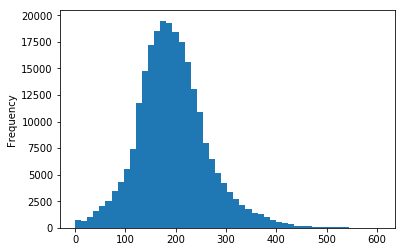
4. Make an histogram to see the values in a different way.
How does this distribution look like?
5. Create another series from the chromosome info and print
the first 10 elements
6. Create a DataFrame starting from the two Series and print
the first 10 elements
7. For each chromosome, get the average insert size of the
paired aligned to it (hint:use group by).
8. Make a box plot of the average insert size per chromosome.
Show/Hide Solution
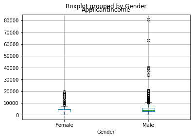
- Download the train.csv dataset. As the
name says it is a .csv file. The file contains information regarding
loans given or refused to applicants. Information on the gender,
marital status, education, work and income of the applicant is
reported alongside the amount and length of the loan and credit
history (i.e. 0 if no previous loan was given, 1 otherwise). Open it
in a text editor or excel and inspect it first. Then, answer the
following questions (if you have any doubts check
here):
- Load it into a pandas DataFrame (use column
Loan_IDas index. Hint: use parm index_col). - Get an idea of the data by visualizing its first 5 entries;
- How many total entries are present in the file? How many males and females?
- What is the average applicant income? Does the gender affect the income? Compute the average of the applicant income on the whole dataset and the average of the data grouped by Gender. How many Females have an income > than the average?
- How many loans have been given (i.e. Loan_Status equals Y)? What is the percentage of the loans given and that of the loans refused?
- What is the percentage of given/refused loans in the case of married people?
- What is the percentage of given/refused loans in the case of applicants with positive credit history (i.e. Credit_History equals 1)?
- Load it into a pandas DataFrame (use column
Show/Hide Solution
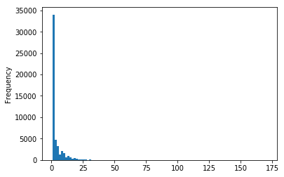
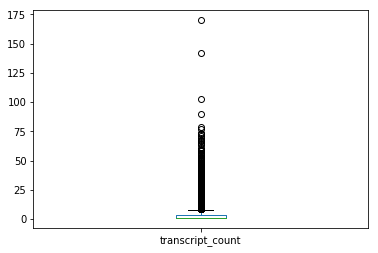
- [Thanks to Stefano Teso] DNA transcription and translation into proteins follows this schema:

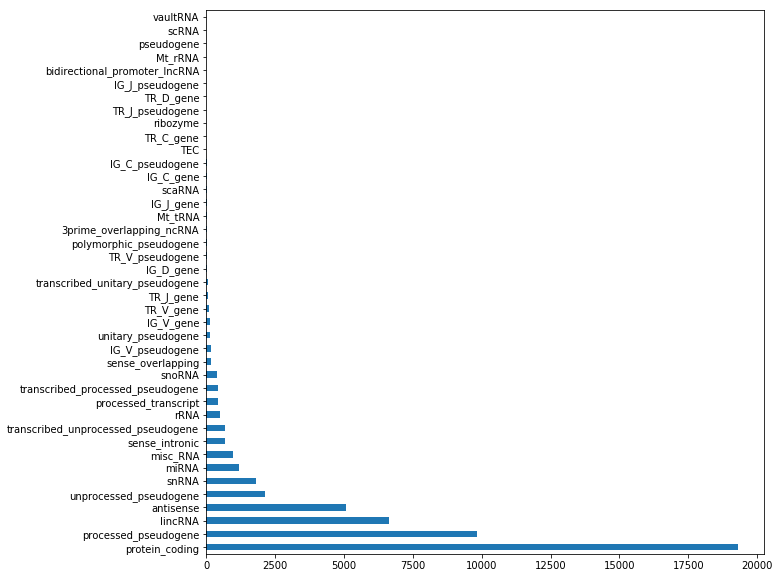
The file gene_table.csv is a comma separated value file representing a summary of the annotation of several human genes based on the Ensembl annotation. For each gene it contains the following information:
gene_name,gene_biotype,chromosome,strand,transcript_count
where gene_name is based on the HGNC
nomenclature. gene_biotype represents the biotype (refer to
VEGA
like protein_coding, pseudogene, lincRNA, miRNA etc. chromosome is
where the feature is located, strand is a + or a - for the forward
or reverse strand and transcript_count reports the number of
isoforms of the gene.
A sample of the file follows:
TSPAN6,protein_coding,chrX,-,5
TNMD,protein_coding,chrX,+,2
DPM1,protein_coding,chr20,-,6
SCYL3,protein_coding,chr1,-,5
C1orf112,protein_coding,chr1,+,9
FGR,protein_coding,chr1,-,7
CFH,protein_coding,chr1,+,6
FUCA2,protein_coding,chr6,-,3
GCLC,protein_coding,chr6,-,13
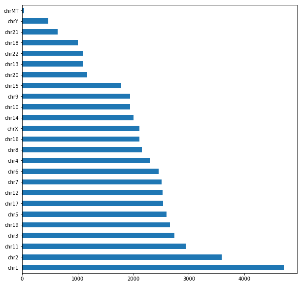
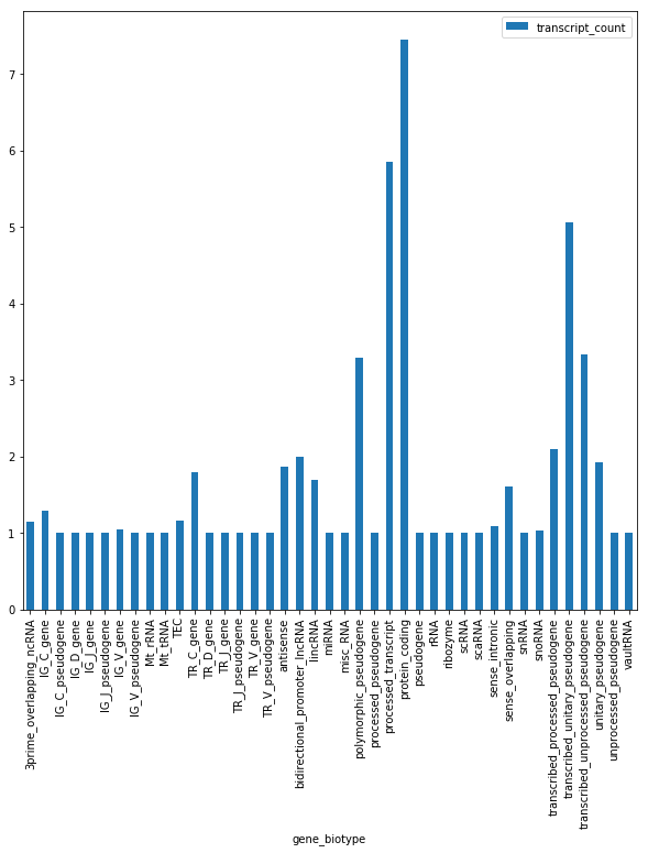
Write a python program that: 0. Loads the gene_table.csv in a DataFrame (inspect the first entries with head to check the content of the file); 1. Computes the number of genes annotated for the human genome; 2. Computes the minimum, maximum, average and median number of known isoforms per gene (consider the transcript_count column as a series). 3. Plots a histogram and a boxplot of the number of known isoforms per gene 4. Computes the number of different biotypes. How many genes do we have for each genotype? Plot the number of genes per biotype in a horizontal bar plot (hint: use also figsize = (10,10) to make it visible; 5. Computes the number of different chromosomes 6. Computes, for each chromosome, the number of genes it contains, and prints a horizontal barplot with the number of genes per chromosome. 7. Computes, for each chromosome, the percentage of genes located on the + strand 8. Computes, for each biotype, the average number of transcripts associated to genes belonging to the biotype. Finally, plots them in a vertical bar plot
Show/Hide Solution
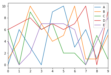
- Write a function that creates and returns a data frame having columns
with the labels specified through a list taken in input and ten rows
of random data between 1 and 100.
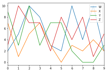
- Create two random DataFrames one with labels l = [“A”, “B”, “C” ,”D”,”E”] and l1 = [“W”, “X”,”Y”,”Z”]
- Print the first 5 elements to inspect the two DataFrames and plot the valuse of the two DataFrames;
- Create a new Series S1 with values: [1, 1, 1, 0, 0, 1, 1, 0, 0, 1]. Get the Series corresponding to the column “C” and multiply it point-to-point by the Series S1 (hint use: Series.multiply(S1))
- Add this new series as a “C” column of the second DataFrame.
- Merge the two DataFrames based on the value of C. Perform an inner, outer, left and right merge and see the difference
Show/Hide Solution